L-VIWO: Visual-Inertial-Wheel Odometry based on Lane Lines
In the process of autonomous vehicle localization, road markings such as lane lines are frequently employed in schemes that match semantic information derived from HD-map a priori maps and integrate GNSS. In comparison to the direct odometer method, the cumulative error can be significantly reduced, and the positioning accuracy can reach the decimeter level. Nevertheless, the production of a priori maps necessitates the expenditure of considerable resources. The article what we‘ll talk presents a method that does not rely on a priori maps and employs lane lines for positioning correction, thereby enhancing the accuracy of the positioning over the conventional VIO scheme.
Overview
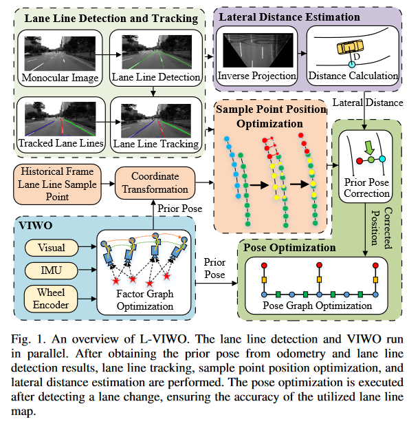
The method proposed in this article is a lane line assisted odometer positioning method. That is, the lane line extraction and tracking are performed in parallel during the odometer operation, and then the position information provided by the odometer is used to assist the optimization of the lane line building map, and the joint map optimization is executed when a vehicle is detected crossing the line. The primary contribution of this thesis is the development of a lane line building graph and a lane line-assisted localization method.
Extract and Tracking of Lane Lines
In this article, the authors have elected to utilize the LaneATT methodology for the extraction of lane lines, employing lane line sample points as a means of representing the lane lines themselves. In this context, the term “lane line sample points” refers to a method of modeling lane lines using a series of points, which are subsequently made continuous through curve fitting. This approach facilitates the calculation of the lateral distance between the vehicle and the lane line,. Moreover, the authors demonstrate that this lane line modeling approach is consistent with the format of the lane lines extracted by the deep learning network, which means that it can be directly embedded into most trained lane line extraction networks.
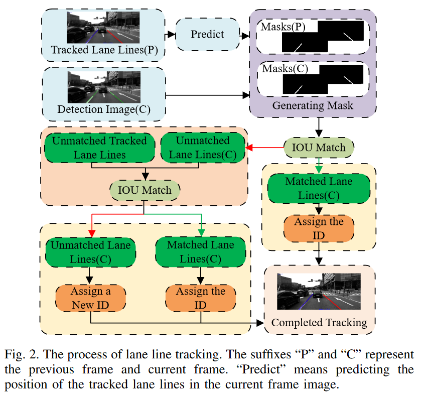
In the tracking part, the article chooses to project the pixel feature points of the k-1 frames into the image of the k frames using the known positional information, compute $IOU$ with the lane lines detected in the k frames, and construct the cost matrix $Cost$.
\[I O U_i^j=\frac{\operatorname{mask}_D^i \cap \operatorname{mask}_T^j}{\operatorname{mask}_D^i \cup \operatorname{mask}_T^j} \tag1\]where $i$ and $j$ are lane line IDs, and $D$ and $T$ denote the current and past frames, respectively. The values of union and intersection are determined by the number of pixels in the corresponding region masks.
\[\operatorname{cost}_i^j=1-I O U_i^j \tag2\] \[\operatorname{Cost}=\left[\begin{array}{cccc} \operatorname{cost}_1^1 & \operatorname{cost}_1^2 & \cdots & \operatorname{cost}_1^n \\ \cos t_2^1 & \operatorname{cost}_2^2 & \cdots & \operatorname{cost}_2^n \\ \cdots & \cdots & \cdots & \cdots \\ \operatorname{cost}_m^1 & \operatorname{cost}_m^2 & \cdots & \operatorname{cost}_m^n \end{array}\right] \tag3\]This is an assignment problem, and the article chooses to use the Hungarian algorithm to solve it.
Hungarian algorithm
The Hungarian algorithm is an assignment problem, that makes the total COST obtained from the final assignment reach a very small value, which is common in mathematical modeling, target tracking and other fields. In this example, first we have to 0-complete the matrix so that the rows and columns are the same.- Step1. Select the smallest element in each row and subtract it from each element in that row.
- Step2. select the smallest element of each column and subtract it from each element of that column.
- Step3. Cover all zeros in the resultant matrix using the minimum number of horizontal and vertical lines. If it is equal to the order of the matrix get the best allocation, if not then proceed to the next step.
- step4. Find the smallest element that is not covered by horizontal or vertical lines. Subtract that element from all the uncovered numbers and add k to all the elements that are covered twice.
The specific steps are shown in the figure.
Lane Line Map Creation
The article suggests that directly stitching lane lines after matching can accumulate errors. Therefore, a certain degree of correction stitching is performed using the portions that may be repeatedly observed between adjacent frames. The specific method is as follows.
First, the IPM(Inverse Perspective Mapping) model is used to project the new lane line sample points into the vehicle coordinate system. Simultaneously, a transformation matrix is applied to project the historical lane line sample points into the vehicle coordinate system as well. By placing both sets of points in a unified coordinate system, subsequent calculations and processing are facilitated.
IPM model
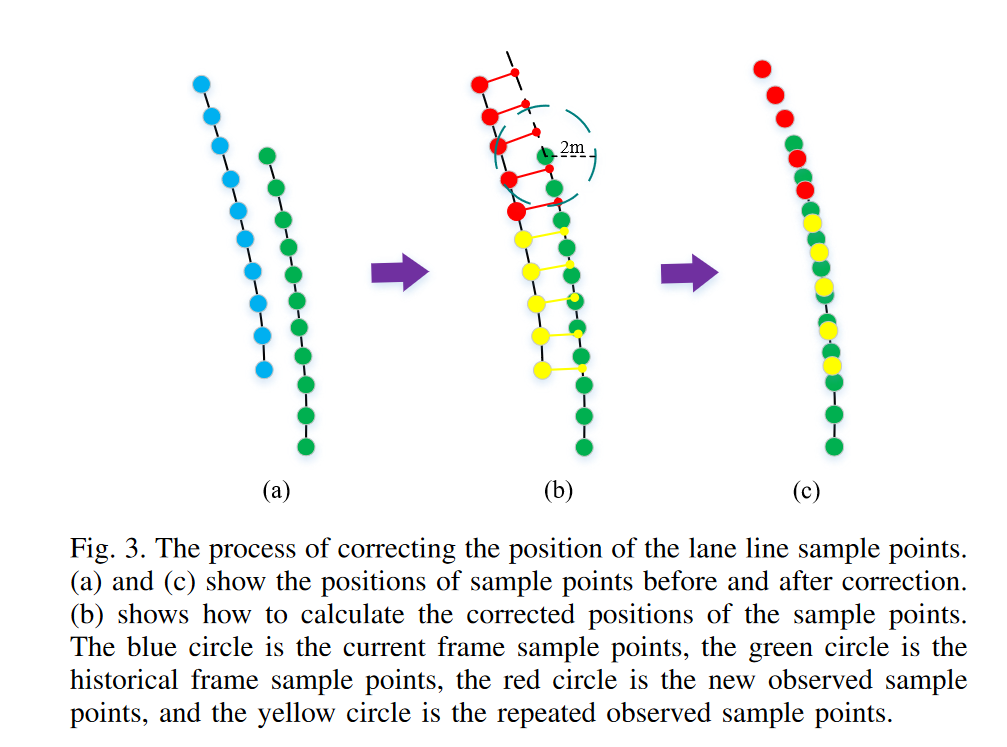
IPM is Inverse Perspective Mapping,which is generally used to eliminate perspective effects, ensuring that parallel lines remain parallel, resulting in a top view in the vehicle coordinate system.The article doesn’t stitch directly, so how is it done? As you can see in Fig. 3, for repeatedly observed sample points the vertical point is taken as the correction position, and for newly observed sample points its weighted the lateral offset of each repeated sample point accumulated to the original coordinate point coordinates, the weighting is mainly considered $X_v$, which is due to the fact that considering that the scale restoration accuracy of the IPM model decreases with distance as the distance increases and decreases
\[\left[\begin{array}{l} X_v^{\prime} \\ Y_v^{\prime} \\ Z_v^{\prime} \end{array}\right]=\left[\begin{array}{c} X_v \\ Y_v \\ 0 \end{array}\right]+\alpha_1\left[\begin{array}{l} a_1 \\ b_1 \\ c_1 \end{array}\right]+\alpha_2\left[\begin{array}{l} a_2 \\ b_2 \\ c_2 \end{array}\right]+\cdots+\alpha_n\left[\begin{array}{l} a_n \\ b_n \\ c_n \end{array}\right] \tag 4\] \[\alpha_j=1-\frac{X_v^j}{\sum_{i=0}^{i=n} X_v^i} \tag5\]where $\begin{bmatrix}X_v &Y_v & 0\end{bmatrix}^T$ and $\begin{bmatrix}X_v’ &Y_v’ & Z_v’\end{bmatrix}^T$ represent the positions of the sample points before and after correction, respectively. $\begin{bmatrix}a_j&b_j & c_j\end{bmatrix}^T$ is the translation vector from the repeatedly observed sample point to the corrected position.
After that, this part also corrects the farther lane lines. It believes that the curvature of the lane lines should be consistent, so the closer one is used to correct the farther one. This part will not be discussed here.
Lane-based Pose Correction
Each time the vehicle detects a lane change (The article does not explain how the lane change is done, but it is speculated that the sign of the detected lane line in the vehicle coordinate system has changed), the vehicle’s lateral distance and lane line map are used to optimize the posture.
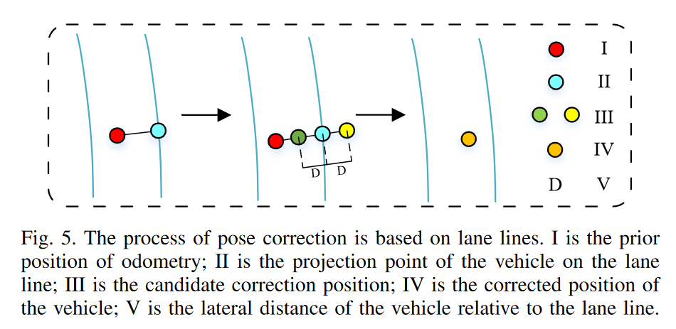
First, the lane sampling points are fitted into a fourth-degree curve. Then, a vertical line is drawn from the vehicle’s position obtained from the odometer to the corresponding lane line, and the intersection point is determined. Next, along the vertical line, we search for a position at a distance equal to the lateral distance from the intersection point. The position to the left of the lane line is chosen as the corrected position of the vehicle. This part is a bit convoluted; I understand it this way: the lateral distance comes from the lane line, while the lateral distance of the vertical line drawn from the vehicle position is obtained from the odometer. The author chooses to consider both methods comprehensively.
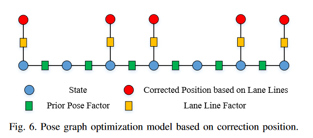
After that, the article constructs a graph optimization by comprehensively considering the constraints of the odometer and the vehicle correction position we just obtained. The objective function and residual factor are following,
\[\chi^*=\arg \min _\chi\left\{\sum_{(i, j) \in O}\left\|O_{i j}\right\|^2+\sum_{(i) \in L}\left\|L_i\right\|^2\right\} \tag 6\] \[O_{i j}=\left[\begin{array}{c} \left(q_i^o\right)^{-1}\left(p_j^o-p_i^o\right)-\left(q_i^l\right)^{-1}\left(p_j^l-p_i^l\right) \\ \left(\left(q_i^o\right)^{-1} q_j^o\right)^{-1} \otimes\left(\left(q_i^l\right)^{-1} q_j^l\right) \end{array}\right] \tag7\] \[L_i=p_{X_i}^l-p_i^l\tag8\]In Formula $(7)$, The first term is the translation residual represented by the quaternion, and the second term is the rotation residual. Formula $(8)$ is also easy to understand, which is the corrected position minus the optimized variable.
Summary
The article does not provide open-source code, and I have not reproduced the results, so I won’t include any images. The experimental section of the paper not only demonstrates the results of L-VIWO but also tests the lane line-assisted localization method using open-source solutions like ORB-SLAM3 and VINS-FUSION, showing some improvement in localization accuracy. In the time complexity analysis, due to parallel processing, the system’s runtime only increased slightly, suggesting it can operate in real-time at over 10 Hz. However, in practice, the testing platform used an RTX 3060 GPU, leading to increased computational costs. Additionally, the KAIST urban dataset used in the study is a city road dataset, but the paper does not discuss scenarios involving special weather conditions or damaged lane lines.
Finally,The author of the paper wrote in the summary:In future work, we will consider constraints from other road signs to improve our system further.
Reference