Numerical Analysis: Polynomial interpolation

In engineering problems or scientific experiments, we sometimes face the following problem: we can only measure the function value or derivative value of a function $f(x)$ at a few points, but we want to get the value of the function at other points. Then we can “create” a function $y(x)$, and approximate the function $f(x)$ on the premise of ensuring that it passes through these known function points. If we use algebraic polynomials, then it is called polynomial interpolation.

When I first learned polynomial interpolation, I was a little confused about interpolation and fitting because both were to obtain a function. But in fact, it is only necessary to clarify that interpolation is to ensure that the function points are passed, while fitting is to minimize the difference between the predicted value and the actual observed value of the model at all data points by constructing an error function.

The following introduces several polynomial interpolation methods.

Lagrange polynomial

Method

The idea of Lagrange polynomial is very clear. Since it is required to ensure that it passes through these known function points, can I add a weight function to the function values of all points, so that when $x = x_i$, this term is 1, otherwise it is 0, so that the condition can be met.

\[y(x) = \sum_{j = 0}^nl_j(x)f(x_j) \tag 1\] \[l_j(x) =\left\{ \begin{array}{rcl} 1 & & {i = j}\\ 0 & & {i \neq j}\\ \end{array}\right.\quad i,j = 0,1,\cdots,n \tag 2\]

Then the question becomes how to define an interpolation polynomial $l_j(x)$. As for the construction idea, we can know from formula $(2)$ that for each weight function, there must be $n-1$ zero points. Then the polynomial comes out, and at the same time, it is required to be normalized. Then the result is obvious. It is given here directly. You can substitute it into the calculation yourself. It is basically no problem.

\[l_j(x) = \frac{\prod_{i = 0}^{j-1}(x - x_i)\prod_{i = j-1}^{n}(x - x_i) }{\prod_{i = 0}^{j-1}(x_j - x_i)\prod_{i = j-1}^{n}(x_j - x_i)} \quad j = 0,1,\cdots, n \tag 3\]

There is actually a small problem with formula (3). If there are two identical points among the known function points, and all points are in the form of (1, 2), (1, 2), (2, 3) and we need to interpolate, then we will construct:

\[l_1(x) = \frac{(x - 1)(x - 2)}{(1 - 1)(1 - 2)} \tag 4\]

Obviously, a problem has occurred: $(1 - 1)$ in the denominator will be zero, which makes the basis polynomial $l_1(x)$ undefined, so Lagrange interpolation requires that the inserted nodes should be mutually exclusive, so there is no problem at all, and the interpolation polynomial is unique at this time.

Error Analysis

The interpolation function has been constructed. How to evaluate the effect of the interpolation function? It is actually very simple. Just subtract it:

\[E(x) = f(x)-y(x) \tag 5\]

Regarding $E(x)$, the derivation process here will not be repeated, only the derivation idea is given: first construct a function about $f(z)-y(z) = k(x)\prod_{i = 0}^n( z - x_i)$. When passing through the interpolation point, the left side minus the right side equals zero. Then take the derivative. Because there are $n + 2$ zero points, there is at least one zero point after taking the $n + 1$ derivative. Then we get $k(x)$, then we can get the analytical form of $E(x)$:

\[E(x) = \frac{f^{n+1}(\zeta)}{(n+1)!} \prod_{i = 0}^n(x - x_i) \quad \zeta\in(a,b) \tag6\]

Newton Polynomial

Lagrange Polynomial interpolation idea is simple and easy to use, but when we need to add new interpolation nodes, we will find that we need to reconstruct the interpolation function. Here is another idea:

\[y(x) = a_0 + a_1(x - x_0) + \cdots +a_n(x - x_0)(x - x_1)\cdots(x - x_n) \tag 7\]

This form of power-raising ensures that every time we add a new node, we only need to accumulate new items on it.

Substituting into the original interpolation function, we can get the value of $a_i$, that is:

\[f_0 = a_0 \\ \frac{f_1 - f_0}{x_1-x_0} = a_1 \\ \frac{\frac{f_2 - f_0}{x_2-x_0} - \frac{f_1 - f_0}{x_1-x_0}}{x_2-x_0} = a_2 \\ \vdots \tag8\]

In this way, the value of each parameter can be obtained by step-by-step calculation.

In order to calculate more elegantly, we define difference quotient:

\[f[x_0, x_k] = \frac{f_k - f_0}{x_k - x_0} \\ f[x_0,x_1, x_k] = \frac{f[x_0, x_k] - f[x_0, x_1]}{x_k - x_1}\\ \vdots \\ f[x_0,x_1,\cdots,x_{k-1}, x_k] = \frac{f[x_0,x_1,\cdots,x_{k-2}, x_k] - f[x_0,x_1,\cdots,x_{k-1}]}{x_k - x_{k-1}} \tag9\]

Obviously, by mathematical induction:

\[a_k=f[x_0,x_1,\cdots, x_k] \quad k = 1,2,\cdots, n \tag{10}\]

In fact, by comparing the leading coefficients of Newton Polynomial and Lagrange Polynomial, it can be proved that the difference quotient $f[x_0,x_1,\cdots, x_k]$ has nothing to do with the order of the nodes; Newton Polynomial and Lagrange Polynomial are also equivalent.

\[f[x_0,x_1,\cdots, x_k] =\frac{f^{j}(\zeta)}{(j)!}\quad \zeta\in(x_0,x_j) \tag{11}\]

Convergence conclusion

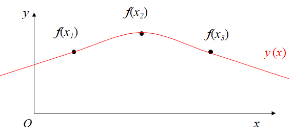
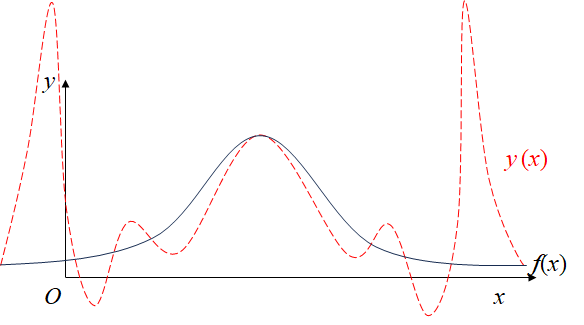
1. Node encryption does not necessarily guarantee that the interpolation function between two nodes can better approximate the function.

2. Involving only the values of the nodes can easily cause the Runge phenomenon of $y_1$ in Figure 1, and the function value fluctuates greatly.

Hermit interpolation

To solve the Runge phenomenon, we only need to add derivative constraints, so that our interpolation function will be as smooth as the original function:

\[\left\{ \begin{array}{rcl} y(x_j) =f(x_j) & & {j = 0,1,\cdots,n}\\ y'(x_j) =f'(x_j) & & {j = 0,1,\cdots,r}\\ \end{array}\right. \tag{12}\] \[y(x)= \sum_{j = 0}^n\alpha_j(x)f(x_j) +\sum_{j = 0}^r\beta_j(x)f'(x_j) \tag{13}\]

The derivation of $\alpha_j(x)$ and $\beta_j(x)$ is also very interesting, but it requires too many formulas. You can refer to

https://zhuanlan.zhihu.com/p/694562765

Result is:

\[f(x)=\sum_{j=0}^n \alpha_j(x) f\left(x_j\right)+\sum_{j=0}^n \beta_j(x) f^{\prime}\left(x_j\right) +\frac{\left[p_{n+1}(x)\right]^2}{(2 n+2)!} f^{(2 n+2)}(\zeta), \quad \zeta \in(a, b) \tag{14}\] \[\alpha_j(x)=\left[1-2\left(x-x_j\right) l_j^{\prime}\left(x_j\right)\right] l_j^2(x), \quad j=0,1, \cdots, n \tag{15}\] \[\beta_j(x)=\left(x-x_j\right) l_j^2(x), \quad j=0,1, \cdots n \tag{16}\]