Numerical Analysis: Solve linear Equations
Regarding the numerical solution of linear equations, there are four main cases for discussion. Finally, let’s analyze the error topic.
\[Ax=b \tag1\] \[\begin{bmatrix}a_{11} & a_{12} & \cdots & a_{1n} \\ a_{21} & a_{22} & \cdots & a_{2n} \\ \vdots & \vdots & \ddots & \vdots \\ a_{n1} & a_{n2} & \cdots & a_{nn}\end{bmatrix} \begin{bmatrix} x_1 \\ x_2\\ \vdots \\x_n \end{bmatrix} = \begin{bmatrix} b_1 \\ b_2\\ \vdots \\b_n \end{bmatrix} \tag 2\]Matrix Solving
Gaussian elimination and Gaussian column pivot elimination
Gaussian elimination
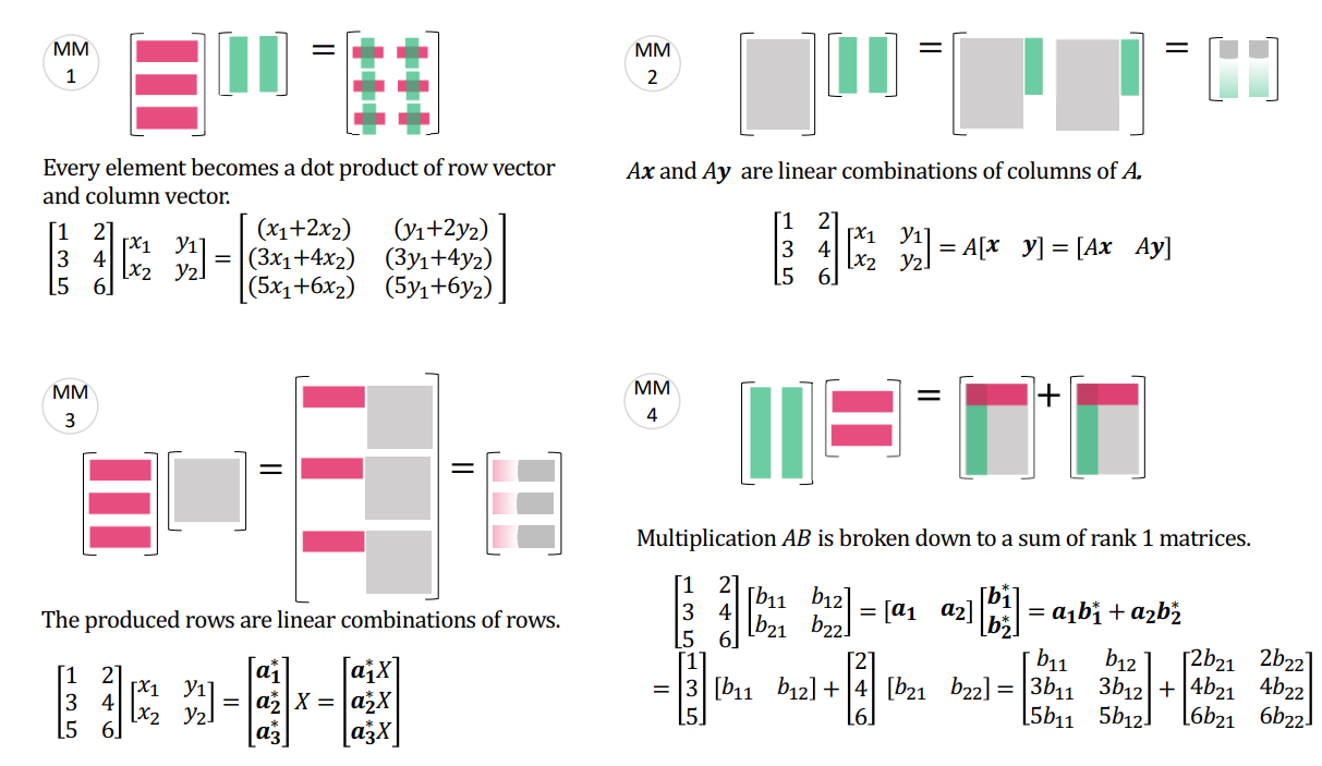
Gaussian column pivot elimination
Regarding the column pivot, the main consideration is the numerical problem in the computer calculation process. For a linear equation system of the form
\[\begin{bmatrix}0.3*10^{-10} & 1\\ 3 & 4\end{bmatrix} \begin{bmatrix} x\\y \end{bmatrix} = \begin{bmatrix} 1 \\ 2 \end{bmatrix}\]If you want to perform elimination, the second column of the matrix needs to be subtracted from the first equation and then multiplied by $m_{21}=a_{21}/a_{11}$,This process can easily distort the results. In this example, the coefficient is $10^{11}$. This is obviously inappropriate, so naturally, the larger the divided value is, the better, and the largest one selected is the column pivot.
Decompose and then solve
LU decomposition、cholesky decomposition
lower–upper (LU) decomposition
There are Doolittle decomposition method and Crout decomposition method. Both methods are essentially LU decomposition. The difference is that the former has 1 on the diagonal of the lower triangular matrix (unit lower triangular matrix), while the latter has a unit upper triangular matrix. It is worth noting that LU decomposition can only be performed under the condition that the matrix is non-singular.
Cholesky decomposition
Compared with LU decomposition, Cholesky decomposition extracts the elements on the diagonal of the matrix after LU decomposition into a diagonal matrix.
\[A = LD(D^{-1}U) \tag3\]Of course, when A is a symmetric positive definite matrix:
\[A = LDL^T \tag4\]Then, according to the idea of LU decomposition to solve the equation, we calculate step by step and finally get the solution of x.
ps: This is the improved Cholesky decomposition. Before the improvement, D was divided into the front and back triangular matrices respectively. The principle is the same
*Symmetric positive definite matrix: All eigenvalues are naturally positive. How to understand it, I am not very clear for the time being [OK, task+1, matrix theory also needs to be read]
In fact, these methods are similar to Gaussian elimination method
Iterative solution
The idea of iterative solution of nonlinear equations mentioned above is the same as that of iterative solution of linear equations, which is to rewrite $(1)$ into an equivalent system of equations and then establish the iterative formula:
\[Ax=b \longrightarrow x = Bx + k \\ \longrightarrow x^{i + 1} = Bx^i + k, \quad i = 0,1,2,\cdots \tag 5\]Since it is an iteration, there must be a problem of convergence judgment. Here we only give the conclusion:
The following three propositions are equivalent
- Iteration $x^{i + 1} = Bx^i + k$ converges
- Spectral radius $\rho(B)<1$
- There is at least one matrix subordinate norm such that $\lVert B\rVert<1$
Jacobi Iteration
Following the above idea, the linear equation system $(1)$ is rewritten. First, the non-singular square matrix $A$ is written in the form of a lower triangular matrix + a diagonal matrix + an upper triangular matrix:
\[A = L + D + U \tag 6\]Then the linear equations are:
\[Ax=b \longrightarrow x = -D^{-1}(L + U)x + D^{-1}b\\ \longrightarrow x^{i+1} = -D^{-1}(L + U)x^{i} + D^{-1}b, \quad i = 0,1,2,\cdots \\ \longrightarrow x^{i+1} = (I-D^{-1}A)x^{i} + D^{-1}b, \quad i = 0,1,2,\cdots \tag 7\]The expanded component form is:
\[x^{i+1}_j = \frac{1}{a_{jj}}(b_j-\sum_{m = 1}^{j-1}{a_{jm}x^i_m}-\sum_{m = j+1}^{n}{a_{jm}x^i_m})\quad j = 1,2, \cdots,n; \quad i = 0,1,2,3,\cdots \tag 8\]Gauss-Seldel Iteration
Considering that the first $j-1$ components of the $i+1$th iteration are not used in the Jacobi iteration, the Gauss-Seldel iteration makes full use of this information:
\[x^{i+1}_j = \frac{1}{a_{jj}}(b_j-\sum_{m = 1}^{j-1}{a_{jm}x^{i+1}_m}-\sum_{m = j+1}^{n}{a_{jm}x^i_m}) \tag 9\]In fact, after derivation, it can be found that only the matrix moved has changed:
\[Ax=b \longrightarrow (L + D + U)x = x + b \\ \longrightarrow x = -(D+L)^{-1}Ux^{i} + (D+L)^{-1}b, \\ \longrightarrow x^{i+1} = -(D+L)^{-1}Ux^{i} +(D+L)^{-1}b, \quad i = 0,1,2, \cdots \tag {10}\]Regarding the convergence of the two methods, there are also several ways to judge:
- If the coefficient matrix $A$ is symmetric and positive definite, the Gauss-Seldel method converges.
- If the coefficient matrix $A$ is strictly diagonally dominant, both the Jacobi iteration and the Gauss-Seldel iteration converge
Gradient method
The gradient method is also an iterative solution, which first sets an initial value and then iterates step by step. However, the main reason for pulling it out of a separate category is that, unlike the previous method of writing a non-singular square matrix $A$ as a lower triangular matrix + a diagonal matrix + an upper triangular matrix, it uses formula $(1)$ to define a quadratic function $f(x)$, and uses the equivalence principle to believe that the necessary and sufficient condition for the solution of the nonlinear equation system is that the quadratic function obtains the minimum value.
\[f(x)=\frac{1}{2}(Ax,x)-(b,x) = \frac{1}{2} \sum_{i = 1}^n\sum_{j = 1}^na_{ij}x_{i}x_{j} - \sum_{j=1}^nb_jx_j \tag {11}\]Steepest descent method
The algorithm idea is as follows:
- Take an initial vector $x^0$ at random, and select a direction based on the initial vector so that the function $f(x)$ decreases fastest along this direction at the point $x^0$, that is,
- To perform a one-dimensional search,
And so on.
Conjugate Gradient Method
The steepest descent method is based on the locality of the gradient, which may bend around, which will increase the number of iterations. The method of quickly reaching the target value is derived from the inspiration of the conjugate diameter of the ellipse.
The formula is complicated and will not be listed here.
Error analysis
In engineering, for the linear equation system $(1)$, the matrix $A$ is measured experimentally in most cases, so it is not necessarily accurate. Then it is necessary to consider how the result obtained by solving the problem will change.
The conclusion is given directly.
Spectral condition number
Define the spectral condition number of the matrix $A$:
\[\text{Cond}(A) = \| A\|_2\|A^{-1}\|_2\]The larger the spectral condition number, the greater the error of the solution may be. When the spectral condition number is equal to 1, the state of the equation system is the best.


