Relearn Linear Algebra: the Basic of Matrix
Linear algebra is a compulsory course for every engineering student, and recently, in the study of computer graphics and robotics, I was deeply impressed by its importance and the shallowness of my own study back then, so I re-learned the course and made this record.
Begin from solving equations
The initial lesson of linear algebra typically entails the resolution of equations. For me, the most striking aspect of this subject is the resolution of equations, which is why this time, the process of reacquainting myself with linear algebra also begins with the most fundamental concepts. A concise overview of the introductory material reveals the existence of a system of linear equations:
\[\begin{align} x + y = 1 \tag1\\ 3x + 4y =2 \tag2 \end{align}\]How to find the solution of $x$, $y$ in a system of equations? This is a basic mathematical problem. The first method to consider is to use the variable $x$ in one of the equations to represent $y$, and then substitute this into the other equation to obtain the result. The second method is to use the equation $(1)$ to subtract three times the formula $(2)$, which is to find the value of $y$, and then use this value in an inverse substitution to find the value of $x$. As the scale of the problem increases, the direct solution becomes unfeasible due to the presence of multiple unknowns. In such cases, the matrix serves as an effective representation.
That is, the system of equations can be transformed into the following form:
\[\begin{bmatrix}1 & 1\\ 3 & 4\end{bmatrix} \begin{bmatrix} x\\y \end{bmatrix} = \begin{bmatrix} 1 \\ 2 \end{bmatrix} \tag 3\]There are several methods for solving this equation, including inverting both the left and right sides of the equation simultaneously with respect to the matrix on the left, which is known as the primary row transform. Indeed, the elementary row transforms serve to reiterate the aforementioned The second method from the perspective of the matrix.
\[\left[ \begin{array}{cc|c} 1 & 1 & 1\\ 3 & 4 & 2\end{array} \right] \longrightarrow \left[ \begin{array}{cc|c} 1 & 1 & 1\\ 0 & 1 & -1\end{array} \right]\tag 4\]The solution will be self-evident. This is merely an illustrative example, and I deliberately selected a non-singular matrix to ensure the problem could be solved. In the context of more complex problems, the utility of matrix elimination is even more evident.
Matrix multiplication
When $A$ is an $m \times p$ matrix and $B$ is a $p \times n$ matrix, let $C$ be the product of $A$ and $B$, then:
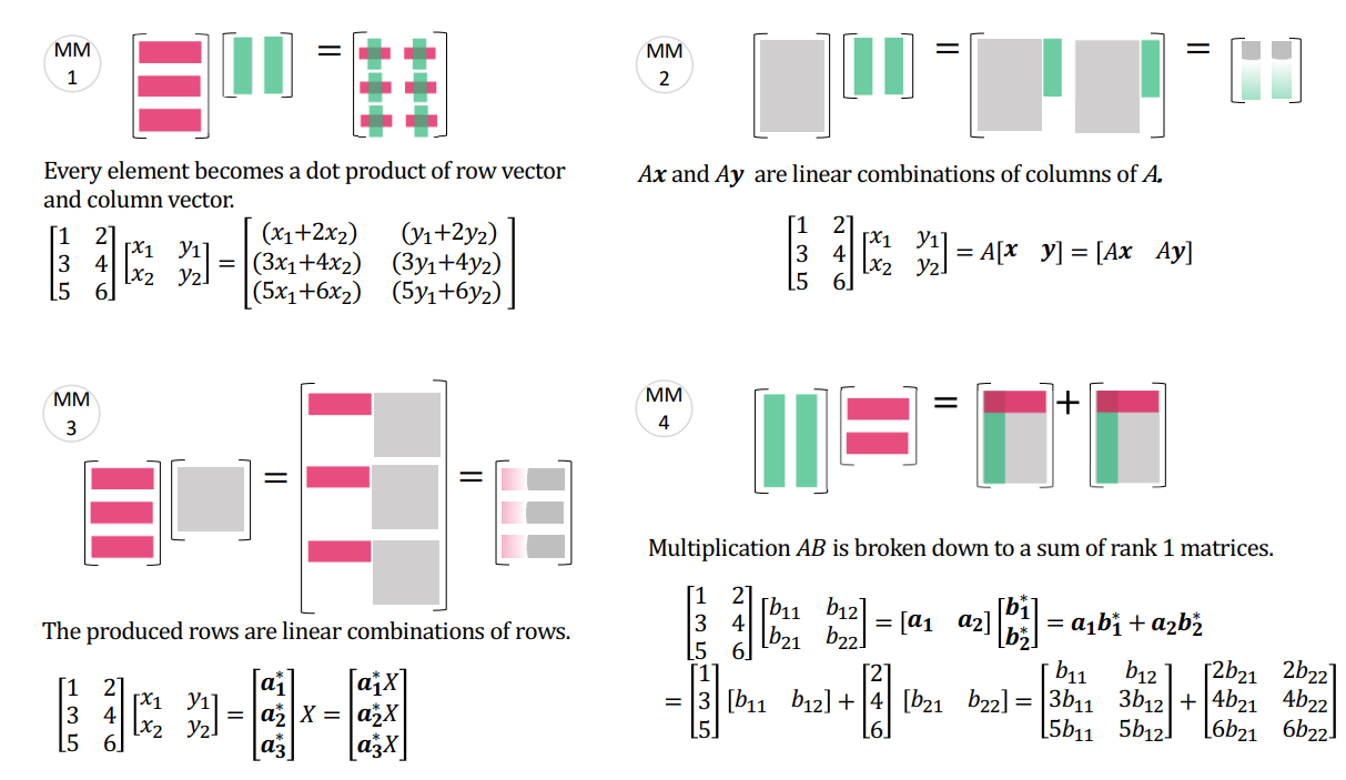
\[(AB)_{ij} = \sum_{k=1}^p{a_{ik}b_{kj}} = a_{i1}b_{1j} + a_{i2}b_{2j} + ···+ a_{ip}b_{pj}\tag 5\]I have exclusively utilized the aforementioned formula for matrix multiplication, a strategy that has consistently enabled me to achieve commendable grades on examinations. While this approach has undoubtedly contributed to my academic success, I have come to recognize that it may have inadvertently obscured the fundamental principles underlying matrix multiplication. The concept of linear transformations is fundamental to the field of matrix multiplication. The following list presents four distinct perspectives on matrix multiplication, which may prove beneficial for further study.
Inverse Matrix
We all know that matrix inverse is also able to solve for the unknowns in $(3)$ because we defined the inverse of a matrix to be a kind of inverse analogous to the inverse in the constant operation, and analogous to the fact that 0 can’t be inverted, and that singular matrices can’t be inverted for matrix inversion either.
\[\underbrace{\begin{bmatrix}1 & 1\\ 3 & 4\end{bmatrix}}_A \underbrace{\begin{bmatrix} a & c\\b &d \end{bmatrix}}_{A^{-1}} = \underbrace{\begin{bmatrix} 1 & 0\\0 & 1 \end{bmatrix}}_I \tag 6\]Gauss-Jordan method
Inverse matrices can be easily solved using the Gauss-Jordan method, which starts by creating an augmented matrix with the inverse matrix to be solved on the left side and the unit matrix. The left-hand side is then converted to a unit matrix using the Gauss-Jordan method, which will cause the right-hand side to be the inverse of the input matrix. The example is still used as a demonstration:
\[\left[ \begin{array}{cc|cc}1&1&1&0\\3&4&0&1 \end{array} \right] \longrightarrow \left[ \begin{array}{cc|cc}1&1&1&0\\0&1&-3&1 \end{array} \right] \longrightarrow \left[ \begin{array}{cc|cc}1&0&4&-1\\ 0&1& -3&1 \end{array} \right] \tag 7\] \[A^{-1}=\begin{bmatrix}4&-1\\-3&1 \end{bmatrix} \tag 8\]The Gauss-Jordan method employs the concept of linear transformations to address the resolution of two distinct systems of equations, ultimately converging them into a single solution.
\[A \times colimn ~ j ~ of ~A^{-1}=colimn ~ j ~ of ~I \tag 9\]